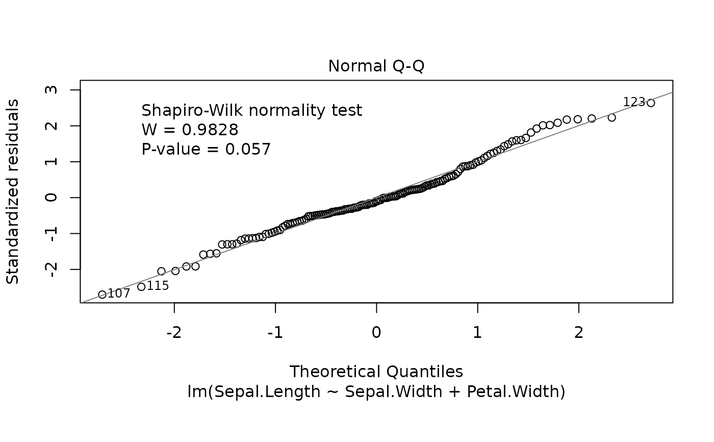
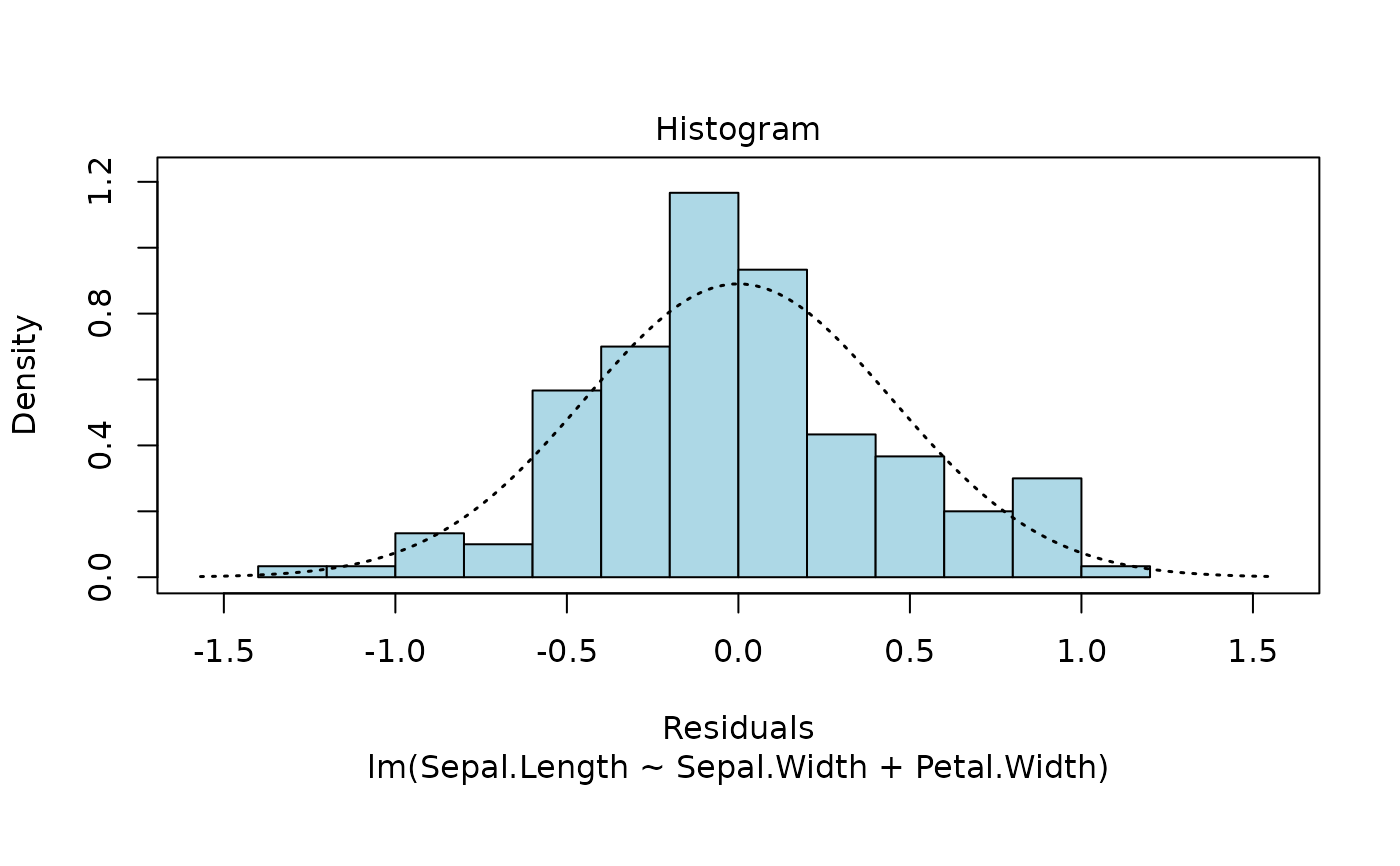
These plots are an extension of the original plots provided by
plot.lm.
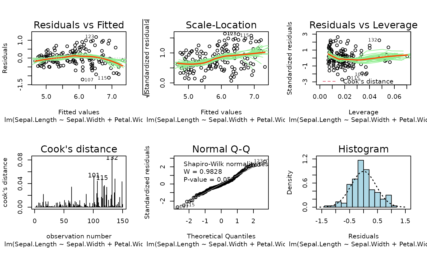
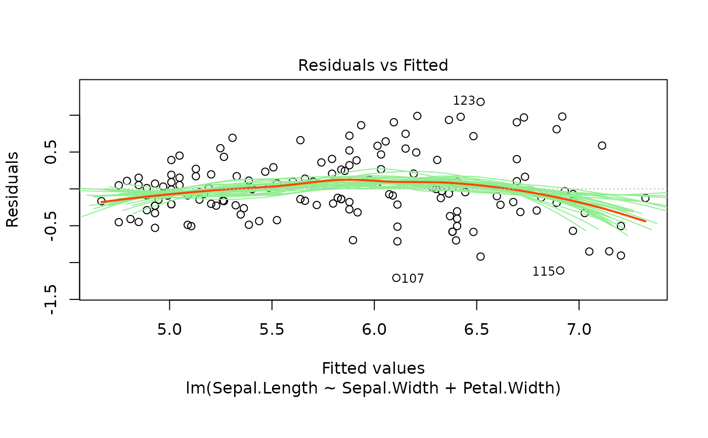
Six plots are currently available: residuals versus fitted,
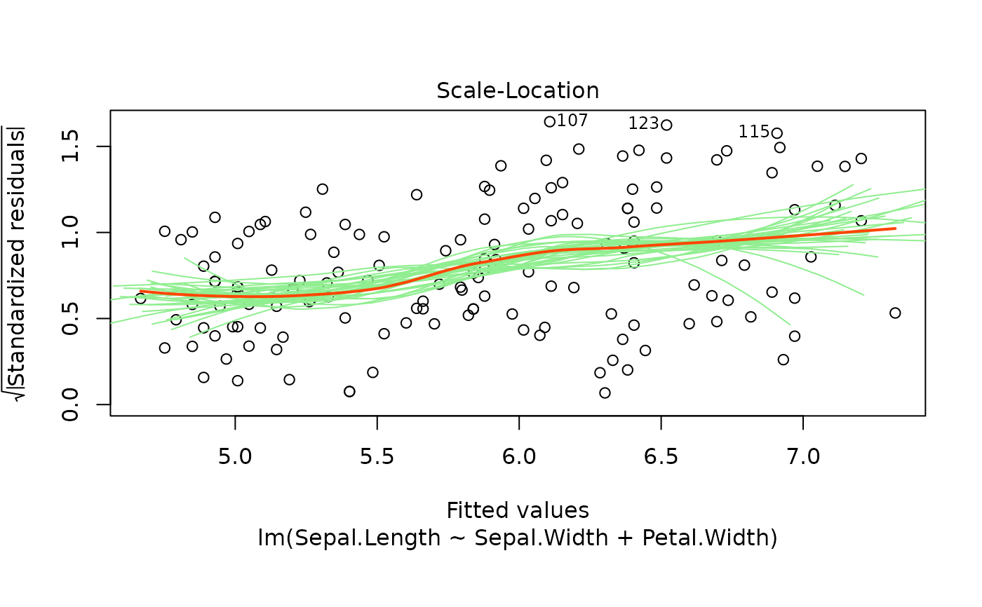
Scale-Location of \(\sqrt{| residuals|}\) against
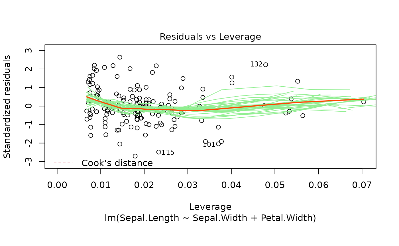
fitted values, residuals against leverages, Cook's distance, Normal
Q-Q plot and histogram of residuals.
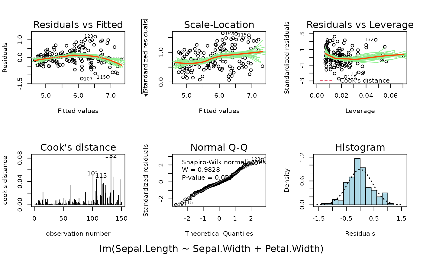
Also provided is the summary plot which shows all diagnostic plots
arranged in a 2 by 3 grid. By default, this is shown first, then each
of the individual plots in turn.
plotlm6(
  x,
  which = 1:6,
  panel = if (add.smooth) panel.smooth else points,
  sub.caption = NULL,
  main = "",
  ask = prod(par("mfcol")) < length(which) && dev.interactive(),
  id.n = 3,
  labels.id = names(residuals(x)),
  cex.id = 0.75,
  qqline = TRUE,
  cook.levels = c(0.5, 1),
  add.smooth = getOption("add.smooth", TRUE),
  label.pos = c(4, 2),
  cex.caption = 1,
  showBootstraps = nrow(x$model) >= 30 && nrow(x$model) < 4000,
  use.inzightplots = FALSE,
  env = parent.frame(),
  ...
)
Arguments
- x
an
lmobject, typically the result oflmorglm. Can also takesvyglmobjects.- which
numeric, if a subset of the plots is required, specify a subset of the numbers
1:6.7will produce a summary plot showing all of the plots arranged in a a grid.1:6will show the summary plot followed by each of the single plots one by one (default).- panel
panel function. the useful alternative to
points,panel.smoothcan be chosen byadd.smooth = TRUE.- sub.caption
common title. Above the figures if there are more than one; used as
sub(s.title) otherwise. IfNULL, as by default, a possible abbreviated version ofdeparse(x$call)is used.- main
title to each plot, in addition to
caption.- ask
logical, if
TRUE, the user is asked before each plot, seepar(ask=.). Ignored when only one plot is being shown.- id.n
number of points to be labelled in each plot, starting with the most extreme.
- labels.id
vector of labels, from which the labels for extreme plots will be chosen.
NULLuses observation numbers.- cex.id
magnification of point labels.
- qqline
logical, if
TRUE, aqqline()is added to the normal QQ plot.- cook.levels
levels of the Cook's distance at which to draw contours.
- add.smooth
logical, if
TRUE, a smoother is drawn to the appropriate plots; see alsopanelabove.- label.pos
positioning of labels, for the left half and right half of the graph respectively, for plots 1--3.
- cex.caption
controls the size of
caption.- showBootstraps
logical, if
TRUE, bootstrap loess smoothers are drawn in the first 4 plots. By default, only drawn for sample sizes of at least 30.- use.inzightplots
logical, if set to
TRUE, the iNZightPlots package will be used for plotting, rather than base R graphics.- env
environment for performing bootstrap simulations (i.e., to find the dataset!)
- ...
other arguments to be passed to through to plotting functions.
Value
No return value; called for the side-effect of producing a plot.
Details
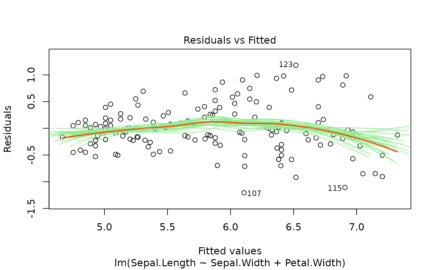
For the residuals versus fitted values plot, we add bootstrapped
smoothers to illustrate variance. The smoother is also added to the
Scale-Location plot.
The Normal Q-Q and histogram plots are taken from the normcheck
function in the s20x package.
See also
Examples
m <- lm(Sepal.Length ~ Sepal.Width + Petal.Width, data = iris)
plotlm6(m, which = 1)
 # the summary grid:
plotlm6(m, which = 7)
 # the default cycles through all 6 plots
plotlm6(m)
